Working through the MRC/WHO 2019-nCoV reports

A team at Imperial College London working with the WHO (I think?) has put together a set of preliminary reports on the 2019 novel coronavirus that can be found here. Here, I will document some of the challenges I personally found while working my way through their analysis. I am not an epidemiologist or a statistician, so this was a great learning experience for me. Any comments I make here could very well be wrong though so let me know.

One reason why reports like this are important is because they allow us to predict how contagious an infectious disease is using a value called the basic reproductive number $R_0$. To predict this, the authors of the reports first generate an estimate of how many cases of the virus were in Wuhan. This analysis is described in Report 2, specifically in the Methods section at the end. They infer this by using the number of confirmed cases detected internationally and estimating the probability of a particular disease case in Wuhan being detected internationally.

Approximation of international detection probability

My first confusion with this analysis comes with the calculation of this probability. In the Methods section, they describe the probability as being calculated as such:

$p = \text{daily probability of international travel} \times \text{mean time to detection of a case}$

or simply

$p = p_{\text{international travel}} \times \bar{t}_{\text{detection}}$

That… doesn’t really make sense as an equation. If the daily probability of travel were 10% (for the sake of discussion), and the mean time to detection was 10 days (the actual estimated time in the report), then you would have a 100% probability of detection oversease. If your daily probability were >10%, then $p$ would be >100%, which makes no sense. Of course the daily probability used in the report was very small (~0.0174%), so that wasn’t an issue, but it frustrated me that I didn’t understand how this simple equation made sense.

Fortunately, my friend Nancy, who is studying epidemiology, was able to clear it up for me. She explained to me that the equation was probably just approximating the probability of a overseases detection by observing that you were more likely to be detected overseas if the detection time was longer. The longer the detection time, the more likely you flew out of Wuhan before you theoretically would have been detected within Wuhan. She added that there are equations like this in epidemiology where approximations can be made assuming the probability of something (e.g. prevalence of a disease) is small.

And then I realized that we could directly calculate the probability that someone leaves the country within the detection timeframe, and it wasn’t a complex calculation, especially since our estimated time to detection is in whole days. The probability can be expressed as the opposite of the probability that one never leaves Wuhan in the detection timeframe:

$p = 1-(1-p_{\text{international travel}})^{t_{\text{detection}}}$

Of course when I used this equation, the probability I got was essentially the same as the approximation used. Interestingly, it looks like this equation can be expanded using the Binomial Theorem, and with a quick Google I realized that the authors of the report used a well-known approximation for estimating binomial probabilities. Fair enough, although it would probably have been a good idea to explain the approximation or something. The way it’s presented in the report makes it look like a definitive calculation and at the very least caused me great confusion .

Confidence Intervals

The second thing that really confused me concerns the calculation of 95% confidence intervals for the estimated number of cases in Wuhan. In the Methods page, the authors write:

Confidence intervals can be calculated from the observation that the number of cases detected overseas, X, is binomially distributed as Bin(p,N), where p = probability any one case will be detected overseas, and N is the total number of cases. N is therefore a negative binomially distributed function of X. The results in Table 1 are maximum likelihood estimates obtained using this negative binomial likelihood function. We now report overall uncertainty as the range spanned by the 95% confidence intervals of the first three scenarios in Table 1.

Just for personal reference, I’m pretty sure that since $N$ is being modelled by the negative binomial distribution, and we know $p$ from the above discussion and $X$ from news reports, then we don’t need to use a maximum likelihood estimate. The estimate of $N$ would just be the expected value (mean) of the distribution, and the confidence interval can be built with the distribution quantiles. I may be wrong about this but I don’t see any other explanation. Some discussion (in Chinese) here.

Also mostly for my own reference, here’s some R code to calculate the mean and CI.

lower <- qnbinom(0.025, size=7, prob=prob)
mean <- n*(1-prob)/prob
upper <- qnbinom(0.975, size=7, prob=prob)

which gives me an estimate of 4022 95% CI [1615, 7507]. This is close to the values in the report ([1700, 7800]), but just off enough that I’m still not sure what’s going on.

My last note is that for calculating the mean of the negative binomial distribution, the equation is $n(1-p)/p$ (Wolfram Alpha) and not $np/(1-p)$ (Wikipedia) simply because the distribution is defined by Wikipedia as the number of successes before a specified number of failures occur, and not the other way around as it is in R.

Hopefully that clears up some parts of Report 2. Again, as of the time of writing this analysis is important because it leads to an expert prediction of $R_0$, which is a big factor to consider when assessing infectious diseases.

Changing Seasons

The first day of spring came almost 3 weeks ago now, but today really seemed like the day winter left for good. I just had my wisdom teeth removed, and I’ve had some time alone with my thoughts to really think about all that’s happened in the last few years.

I started this blog almost 4 years ago now as a sophomore (seriously, why don’t Canadians use this terminology?) studying medical sciences. Back then, I wanted to go to medical school and be a doctor, but it wasn’t really the burning passion that my peers had. It was really just the most obvious path, in my head.

4 years later, I still don’t know what I want to do. I applied to medical school several times now, and whether that will work out in the future is still a mystery. I’m almost done my Master’s in Engineering (!?), and I don’t know if I want to go back to school or not. I mean, I’m basically graduating from grade 17 – 17 years of going to class, having my life completely structured around education.

It’s not all that bad though, because I love learning. There are still so many things I want to learn that I haven’t gotten around to, but I think I’m okay with not returning to school next year. I’m excited to potentially find a job and start making a living. Yeah, your life is still centred around this social construct where you have to go and work 8 hours a day or something. But it’ll be nice to have the rest of the time to really enjoy my life and not worry about the next exam or application.

What is certain is that I will be blogging more (holding myself accountable here). The next few months will be me finishing an internship for my Master’s, and I guess I’ll figure out everything after that as I go. I’m still going to primarily keep this space education/tech based, but I’m going to try and share more personal things too. I have changed in the last 4 years, and I have grown, and I feel that a lot of that personal growth deserves to be described, if only for my sake.

Ontario Graduate Scholarship?

TL; DR - Even though OGS may be paid to you directly, your supervisor (the school) will adjust your funding accordingly so that you will get the same minimum stipend. Your supervisor may choose to give you an extra couple thousand, but you do not get $15,000 on top of your base stipend.

Now that I’m graduating, I’ve reached a crossroads as to where I want to go. As a student in a research-intensive program, one of the obvious choices was to apply for graduate studies at my current school. A masters in Medical Biophysics was always one of my options, but to be honest, it wasn’t very far up on my list. So applying to external funding, like the Ontario Graduate Scholarship (OGS) wasn’t a priority.

However, I let myself be talked into doing it anyways. On the day of the deadline to start the OGS application, my work study supervisor pointed out that it was worth $15,000; I would be a fool to leave that much money on the table without even putting my name into the hat. And so, with 2 hours left before the deadline, I started and finished my graduate application. It was an exhausting process, but I thought I did very well. But the OGS submission deadline was in a week, and I had work to do.

References were emailed, and favours were asked of. Somehow, I pulled together two strong references and began working on a proposal for my potential project, in which I had next to no knowledge of. It was a brave endeavour, and I didn’t expect it to be my best work, but I wasn’t giving up $15,000. Until my friend pointed out to me that I wouldn’t actually be getting an extra $15,000. He linked me to this Reddit thread, where it is stated that OGS is paid to the department.

I figured that this must’ve been some weird UofT quirk. After all, the OGS page at Western clearly states that “the annual value of an award is divided into three equal installments and each is pre-paid to the award holder’s Student Center account at the start of every term”. I wasn’t worried: the language is very clear. However, I asked another friend, and he told me that the $15,000 didn’t go to me. At this point, I was very lost.

I decided to go deeper. Searching for information about OGS itself seemed to be fruitless, since everywhere it states that you get $15,000. It was only when I looked in the “Medical Biophysics Graduate Handbook” that I found this tasty nibblet of fine print (page 18): “For the length of the OGS scholarship – student receives WGRS + OGS + additional support from supervisor to bring minimum stipend to $15,400/yr”.

Are you kidding me? This means that the supervisor does needs to provide much less additional support to bring the stipend to $15,400, which is guaranteed to every masters student in biophysics. In short, this scholarship does not guarantee any monetary benefits to the applicant. Fortunately, it seems like most supervisors in biophysics will “top-up” the stipend by a couple thousand dollars, but this is a far cry from the $15,000 advertised.

I will admit that perhaps, if I had done my research properly (maybe I’m not suited for graduate school after all), I would never have mixed this up. But I also feel that Western, along with seemingly every other school with OGS, has done a terribly poor job in being transparent with the different funding opportunities for graduate students. The webpage is intentionally misleading, and seems like a false hope for students hoping to supplement their stipend. I hope that Western does a better job in the future to better aid prospective graduate students with funding.

Deconvolutions and EPSCs

So at the research lab I’m working in this summer, the field of study is in neuroscience. And while that’s relatively new and unknown territory for me, I have tried my best to learn and to bring my own experiences and skills to the new problems I face.

EPSCs

Part of what I’m doing involves investigating electrical properties of neurons in the spinal cord. Neurons communicate with each other at junctions called chemical synapses. At these junctions, neurotransmitters are released from one neuron (the presynaptic neuron), which causes a change in the receptors on the postsynaptic neuron, causing a flow of ions into the cell. In this way, a neuron receives inputs from many other neurons.

To look at these inputs, the voltage clamp technique is used to hold the membrane potential at a constant level. The current required to keep the constant potential is measured, and the different inputs are represented by spikes, the excitatory postsysnaptic currents (EPSCs). By analyzing the characteristics of these EPSCs (such as the shape of these spikes and their frequencies), we can start to understand the functions of different neurons.

Simulated voltage clamp data

Deconvolutions

However, manual detection and analysis of these EPSCs is tedious and subject to observer bias. In this paper by Pernía-Andrade et al, a method of detecting EPSCs is proposed using deconvolutions.

About Medical Biophysics (part 2)

The last two core third-year courses in the Biophysics program at Western have been keeping me busy this semester, among other things. In the spirit of completeness, here’s an overview of what they’re about:

1. Fundamentals of Digital imaging (3503): Another course split between 4 different professors, covering a very wide range of topics in medical imaging with an emphasis on general concepts that are applicable to many different imaging modalities.

   The first part of the course started with an overview of imaging science and how its role in medicine, including looking at SNR, contrast, and ROC curves. In particular, learning about ROC curves and other ways of quantifying imaging techniques was useful because they were translatable to other things like classifiers in machine learning. Fun fact: the ROC curve originated from the battlefields of World War II, where it was used to quantify enemy detection. Here’s one I generated for my research:

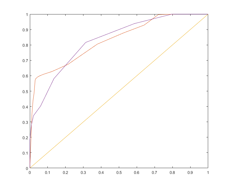   ROC curves of two different red blood cell focus measures

   After that, we learned about more about the actual image capture, and here there was some overlap with one of the sections in optics 3645 (in fact, the same prof taught this part). We learned a bit of the physics and engineering involved in CMOS and CCD sensors, and overall it wasn’t hard at all (I felt like we all lacked the physics background to go in-depth). However, the midterm for this section was really hard for some reason.

   The third section, which I’m currently in, is another overview of MATLAB (it really is used a lot in Biophysics!). I think our prof is doing a really good job with explaining the basics, and he’s focusing on image segmentation techniques which I think is really useful. From my own experience, the majority of my MATLAB usage has been to separate out features from an image, so it’s quite applicable.

   We haven’t started the last section yet, but as I understand it, we will be learning about how imaging is affected by our own perception (the eye as a camera, space perception, …). Not too sure yet.

2. Oxygen Transport (3507): This course hasn’t been the most popular among my peers, and I think a large reason why is because of how silly it seems at times. I mean, why do we need to dedicate an entire course on the diffusion of oxygen? At a first glance, it really just seems like the professor is merely teaching the focus of his research, and not because it serves any educational purpose.

   The course itself focuses on modelling the diffusion of oxygen through different medium and in different geometry using differential equations and other mathematical tools. It’s a little math heavy, and that does turn some people off too. But apart from the actual content, I think it’s an important course because it teaches you how to approach problems in a systematic way (we are taught a “7 steps of problem solving”). While critics say that it’s a little ridiculous that we’re tested on these steps, I think that teaching a general problem solving framework is a really good idea, and applying this technique to mathematical modelling problems helps place the techniques into a biophysical context. Oxygen transport might not be very important to most people, but learning to develop models to describe biophysical phenomena is a useful skill and feels like a major theme in many of our third year courses (see transport systems, biomechanics, math transforms).

   However, as I do like math more than most in my program, your mileage will definitely vary with this course.

   Full disclosure: I have done research with the professor of 3507.

Final thoughts: From the last two posts, I hope anyone reading them has gotten a good feel of what Medical Biophyics at UWO is like. These are the mandatory courses for everyone in the program (apart from Optics), so I believe it to be quite representative of the program. I feel like while we explore a variety of different topics, one problem is that no single topic is studied at a deep level simply because most people in the program (myself included) lack the sufficient biology, math, physics, or engineering background. Medical biophysics as a field is really the result of many experts in vastly different fields coming together to solve medical problems, so it’s really hard to teach this discipline at an undergraduate level.

I feel that this program will definitely benefit people who are self-directed learners, those who seek to explore things they are interested in on their own. The different courses will definitely teach you to problem solve more than it will give you a rich knowledge of anything in particular (as opposed to modules like Physiology or Microbiology and Immunology). Whether or not that’s what you’re looking for is up to you.